Say no to buffer tasks
This blog looks at the applicability of introducing buffer tasks to a schedule to apply the Theory of Constraints (TOC) and suggests alternatives. The conclusion is that rather than introducing buffer tasks as a sole fix for managing operational uncertainty, it is better to ensure that the appropriate mining rate for the scheduling time frame is being applied and to analyze the mining chain available “stocks” in the schedule (and maintain those stock levels as a focus in the scheduling process).
Background
One of our Deswik software users had been discussing with us the applicability of the TOC to their mining schedule. The suggestion from their site was to add a buffer task (time buffer) of a two-week duration prior to the blasting of each stope.
We identified a few issues with this:
- Potential to push out production for a task that does not exist
- Extra complexity to an already complex schedule
- Additional costs associated with creating buffer
- Introducing a task/delay to the short to mid-term schedule that does not exist in the long-term schedule.
Our alternative suggestion was to first do stocks reporting and ensure that they were using resource levelling in the schedule using appropriately selected productivities that match the schedule timeframe being developed. Only then should judiciously-used buffer tasks be considered (if at all – as dependency lag times may be a more appropriate approach than introducing another scheduling task).
Tracking stock levels is far more appropriate
In the author’s opinion, an inserted time buffer of two weeks in the schedule for every single stope blast defeats the purpose of efficient, flexible and reliable work schedules. It may be preferable to blast stope A tomorrow, and stope B in four weeks’ time (so an average of 2 weeks each). The author has not seen TOC applied to schedules per se. It tends to be applied to the operations (to which scheduling is a supporting activity), although the two obviously inter-link. It may be possible to recognize and evaluate a “resource” bottleneck via a schedule, and then be able to justify more or different resources by showing the effect through the schedule.
The author’s experience and reading suggest that ensuring that there are “stocks” in the mining process that act as buffers supporting the system bottlenecks is a far better approach. The stock levels however can be expressed as an equivalent time period rather than just a tonnage level. For example, blasted ore stocks equivalent to two months production may be required at all times (in the schedule).
de Kruijff, Slade and Kennedy (2006) discusses an interesting journey that Mount Isa Copper Operations (MICO) went through in ensuring that they achieved an increased sustainable production rate.
The paper discusses how MICO was in a situation where the tonnage being achieved at the end point of the mining system (delivery to the mill) was well below nameplate capacity. It was also observed that the mining system was operating with an extraordinarily high standard deviation. The deviations in the individual mining unit operation performances were too high for inventory capacity levels to compensate between nodes in the system. The combination and sequential nature of the system meant that each delay or production shortfall at each stage compounded further delays downstream. As each node was dependent on the one preceding it for supply and the one following it for surge capacity, the delays that propagated up and downstream within the overall system were significant.
The solution MICO implemented was based on a process that divided the mine at the stope drawpoint into upstream and downstream processes from the stope drawpoint, and ensuring that there were strategically planned and maintained buffer stocks between the upstream and downstream processes thereby decoupling the two parts of the process. Deliberately maintaining two months stock of broken ore across a number of stope locations/sources allowed the dependency between upstream and downstream processes to be broken allowing the downstream to flow smoothly and independently of the supply noise upstream. Similarly, it is noted that in Bloss (2009), a discussion on mine bottleneck management at Olympic Dam, indicates that a broken ore stock level of approximately 2 months is also used as a production buffer.
Stocks levels at the other “nodes” between the mining unit operations prior to the in-stope broken ore were managed (scheduled) to ensure that the broken ore stock level was planned to never be less than two months (which allowed for the coverage to be available for unforeseen events in the mine and any resulting production “hiccups” to be absorbed).
Reducing production volatility
Some research has been done on the relationship of “production variability”, “production volatility” and stock levels maintained in the underground mining process chain.
Peter McCarthy, Chairman Emeritus & Principal Mining Consultant at AMC has stated:
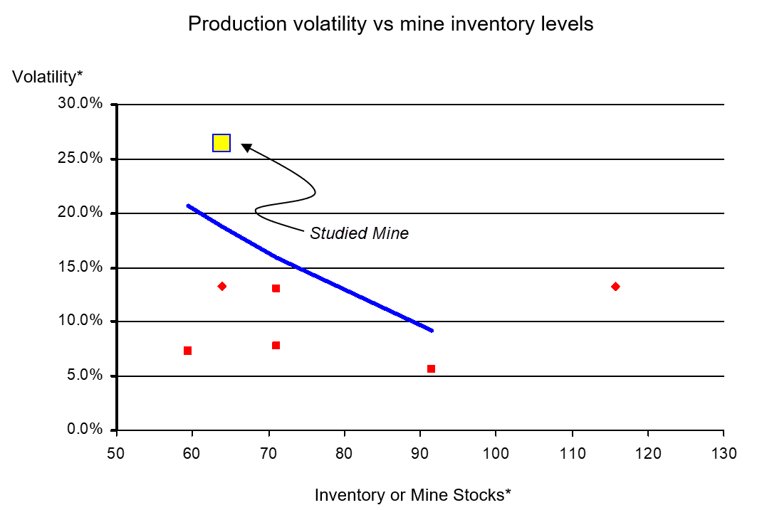
“The more challenging the mining situation the greater the stock levels need to be, including developed (exposed) ore stocks, drilled stocks, broken stocks, and ROM pad stocks. If these stock levels are adequate then volatility can be reduced to a minimum. The mine should be designed so that all stockpiles, including orepasses in an underground mine, have adequate capacity to smooth the short-term surges to a level acceptable for the system as a whole, including ore processing. This is a commonly overlooked requirement.” (McCarthy, 2011)
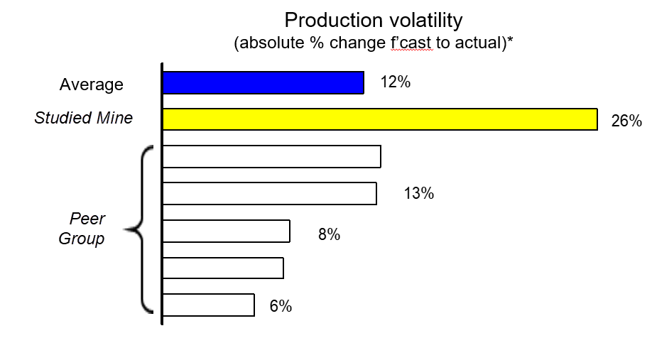
In a benchmarking report produced by AMC for a mine the author was involved in, production volatility was assessed against mine inventory levels for a number of peer mines from the AMC database:
Effect of Adequate Stock Levels
In recognizing that mining unit operations are stochastic rather than deterministic, it is therefore readily understood that as a result, especially in the short-term, bottlenecks can shift from one process to another process in the mining chain depending on availability, utilization, or productivity metrics. In addition, there is always uncertainty about the orebody being mined and the ground being mined in.
The best method of managing this uncertainty and being able to achieve acceptable sustainable long-term performance is to maintain sufficient stock levels between the various unit mining activities to give physical buffers between the various unit operations.
Hall and Harper (2005) give an excellent discussion on how by maintaining adequate ore stock levels it is possible to avoid ore shortages and reduce variability (defined as the difference in the month-to-month planned to actual performance) and volatility (defined as the month-to-month fluctuation in actual performance).
Studies referenced by Hall and Harper (2005) show that the best practice mines achieve an average variability of less than five per cent and a similar average monthly volatility. In contrast the majority of mines shown have an average monthly volatility greater than ten per cent.
The following graph given in Hall and Harper (2005) shows the range of average monthly volatility in ore tonnes mined at a number of mines.
Ore tonnes mined – average monthly variability:
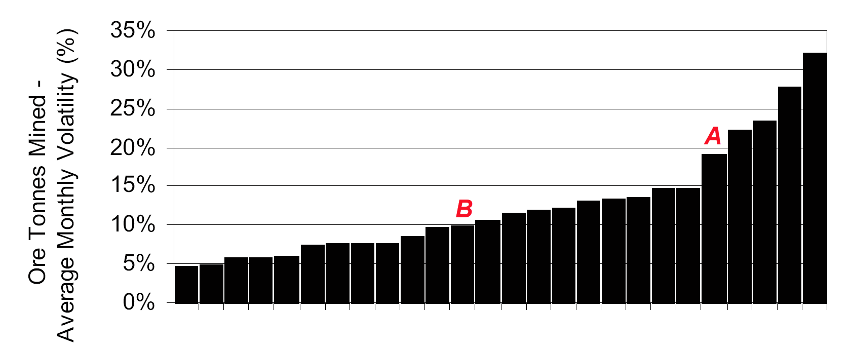
Interestingly two of the points (“A” and “B”) are for the same mine, but at different times. The improved (lower) volatility performance of the mine at time “B” was linked to an increase in ore stocks and available working areas. This “… enabled better utilisation of people and mining equipment, and greater quality control resulting in an improvement in overall mine performance. This [was] demonstrated in measurable terms by a 40 per cent reduction in the underground mining cost per tonne of ore mined while the mine simultaneously achieved planned metal production.” (Hall and Harper, 2005).
Types of Stocks to be Measured
The types of ore stocks that should to be tracked in an underground mine schedule include:
- undeveloped,
- developed,
- drilled,
- broken,
- loaded and hauled,
- hoisted, and
- ROM.
The quantity of ore stocks required for sustainable exploitation of the mineral resource will vary depending on the specific circumstances faced by the operation. It requires analysis of historical data and monitoring of performance as changes are made. It is therefore difficult to make a specific recommendation for any particular operation. Capacities in the mining system and how easily a bottleneck moves between mining unit operations will all have an influence on the size of the stocks. And it is also recognized that maintaining stock levels has a cost. However, Hall and Harper (2005) have some excellent advice on the topic of the costs suggesting that the “value lost through lost production will generally far outweigh the cost of early development. However, the latter is clearly visible as a cost in financial reports, while revenue shortfalls are not.”
Bloss (2009) describes a “debottlenecking strategy [that] was based on the assumption that throughput is prioritized over costs at the bottleneck. This is because throughput gains at the bottleneck are transferred across the whole operation, resulting in a proportional increase in revenue that is commensurate with the proportional increase in throughput at the bottleneck. … There is significant leverage potential for increasing cashflow (revenue less cost) when increasing throughput at the bottleneck”.
It should also be noted when monitoring stock levels, that note should be taken of “available” versus “non-available” stock levels. Having 12 months of drilled ore stocks may not be much use if they are not available due to stope sequencing constraints being such that they cannot be used in the event of a problem, as several undrilled stopes must be taken first for access or geotechnical constraints (unless those stopes are “sacrificed” as unrecoverable).
Other bottlenecks
The main steps in the process of applying a TOC strategy is identifying which of the various operational bottlenecks should be managed as “the bottleneck” (it is easier to manage a single bottleneck in a system), stabilizing and supporting that bottleneck (i.e. managing stock levels such that the bottleneck does not tend to move from that unit operation to other unit operations) and exploiting that bottleneck (maximizing and increasing the throughput through the bottleneck).
As discussed earlier, to avoid the situation of the bottleneck moving rapidly between the various mining unit operations, each of the mining unit operations will need stocks both in front and behind them to act as buffers for short-time scale variances in the mining unit performance.
However, sometimes it is not just the mining unit operations that are bottlenecks, but aspects of the mining operation as a system.
While the author was doing scheduling work for Mt Isa many years ago, it was realized that the combination of stope size and orebody size meant that the number of potentially active stopes became the bottleneck, and changing the size of the stopes (and therefore changing the number of available working faces) changed the nature of that bottleneck. That realization was studied and published in the IMM Transactions (Poniewierski, 2005).
Production rates vs. scheduling time frame
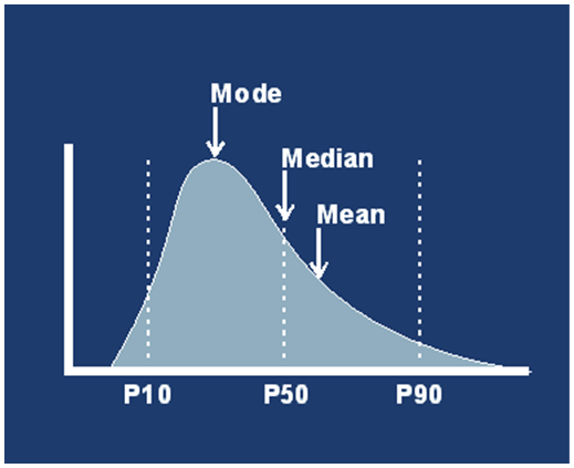
A key issue between long-term schedules and short-term schedules, is that long-term schedules should be using a «mean» rate – a rate derated for the inclusion of the effects of major shut-downs, break-downs and other delays (so effectively it is the mean rate measured or estimated over several years), whereas short-term schedules should usually use «modal» rates as determined by short-term data and excluding effects of major shut-down, break-downs and other unplannable delays. Given the skewed distribution of task rates for most mining activities, the «mean» is usually much less than the «mode» – hence effectively derating for the long-term.
Short-term has to use the modal rate without the effects of longer-term delays built in, otherwise there will be a conflict in resource matching and likely timing of readiness of activity sites, or a mismatch in equipment numbers.
An example of the differences in the use of mean rates versus median and modal rates is given in Resoort (2010), in which the drill and move time data for a raise bore rig drilling stope slots at Kidd mine was analyzed – as shown in the following Figure.
Distribution of raise bore slot drill and move time – Kidd mine (Resoort, 2010):
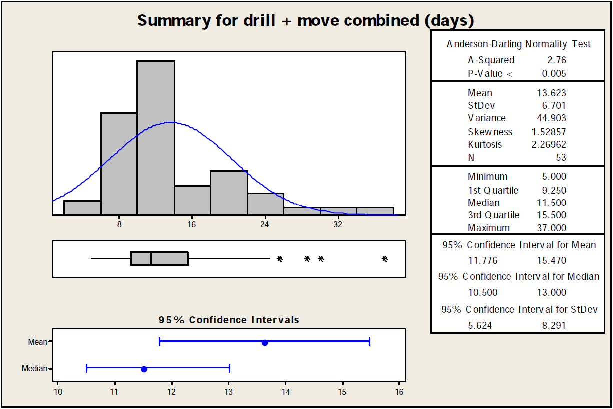
In this example, the median value for the drill and move time for a stope slot is 11.5 days. For 50 per cent of the time it will take less time, 50 per cent of time it will take more time. However, the distribution is skewed to the right, as a result of unplanned events (e.g. the vent bag needed repair; pipes were blown down, etc.), and the mean time was 13.6 days.
The mean result is 18 per cent greater than the median time.
The author suggests that the median or even better – the modal time – is the time that should be used in short-term scheduling. This will be the value most likely to occur, with subsequent short-term plans adjusted for the events that cause the mean to be greater than the median. But for long-term scheduling, it is the mean value that should be used, as “on average” each scheduled stope start time in the long-term mine plan will slip by 2.1 days. The shorter median or modal time should be used in the short-term schedule in order to ensure sites are ready and available when the rig is ready to be moved.
With respect to equipment matching, the example in an open pit would be shovel vs required truck number. In the short-term a shovel can perhaps load say 5 trucks at the «modal» daily loading rate, but at the lower long-term «mean» daily rate (averaged over a year) the shovel would only need 4 trucks “on average” – which if used would mean that the higher «modal» rate would then never be achieved (because not enough trucks were provided).
Scheduling for buffer stocks
Scheduling to maintain buffer stocks is however not a straightforward task. Stock levels are a “result” quantity rather than a driving quantity for a schedule and as such cannot be directly scheduled. In Deswik.Sched stock levels are reported by calculating the difference in flow in and flow out for a period against an inventory. For example, drilled stocks are calculated as the available drill stocks last reporting period (inventory) plus new drilled material (flow in) minus newly blasted material (flow out), rather than targeting the stock level directly. For each schedule run, the resulting stock levels need to be evaluated. If the stock level is not satisfactory then changes need to be made to manage either the flow in or the flow out to increase (or decrease) the stock level being examined.
In long term planning the upstream derived activities associated with stopes, such as production drilling are usually scheduled as «as late as possible» (ALAP) tasks. This task scheduling assignment doesn’t really allow for ease of managing stock levels in a schedule. The timing of some of these upstream activities may need to be moved to a time in the schedule earlier than set as an ALAP task. This may be by judiciously introducing a lag (delay) time on a specific key dependency, introducing a buffer task in a specific location, or just manually moving a task to a “must start by” date, and observing how the stock levels change with these introduced activities (but don’t introduce a blanket lead time, or a blanket buffer task before each stope). Most schedulers however are currently assuming that adequate stocks will be able to be scheduled in the short-term schedule for a given long-term schedule, by derating the resource rates applied.
de Kruijff, Slade and Kennedy (2006) do discuss the use of buffer time in the scheduling used at MICO, but we will contend it should only be used as an adjunct to the use of schedule stock level management and application of schedule time-scale suitable production rates – not as a first pass replacement for these scheduling approaches.
As an adjunct to the management of stock levels and the use of appropriate rates in a long-term schedule it may then be necessary to include a time buffer (as a dependency time lag rather than a new type of activity to add to the schedule).
In short term scheduling – the derived tasks are usually scheduled as «as soon as possible» (ASAP) tasks which if the resources available are adequate will allow stocks to build. The problem is then one of manually managing the allowable levels of the resources for these tasks such that stocks do not become excessive. If sufficient stocks cannot be achieved with a short-term or medium-term schedule, then you have a problem! A problem that may be able to be resolved with extra resources if they can be brought to site.
It is noted that there is often a focus in an operation on the efficient utilization of each and every piece of equipment at a mine site. This can be a value-destroying focus. In order to support a bottleneck, the resourcing around that bottleneck needs to be linked to peak demand at the bottleneck – not the average demand. The equipment itself can be thought of as a “capacity buffer” rather than a physical buffer. Utilization of equipment does not need to be high – but equipment needs to be available when required for supporting throughput through the bottleneck. Remember: “lost production at the bottleneck is lost to the whole system and is unrecoverable” (Bloss, 2009).
One other approach that has been successfully used to help manage the order of tasks that helps with stock levels is a process we’ve called “index-based levelling”, where once an order of stope production has been settled upon, the tasks that lead to each stope via a dependency chain are given an index value based on the order of production. These index values are then set as the priority for the resource doing these tasks. This ensures that any stock that are created are also created in the best locations for maintaining consistent production.
Julian Poniewierski (Fellow AusIMM, CP (Mining))
Further reading
- Bloss, M. 2009, “Increasing throughput at Olympic Dam by effective management of the mine bottleneck” by Martyn Bloss, Mining Technology, vol 118, pp. 33-46.
- de Kruijff, S, Slade, N, and Kennedy, D, 2006. “Improved Mine Throughput Ensures a Sustainable Return on Capital at Mount Isa Copper Operations”, International Mine Management Conference, pp 163-171, October 2006.
- Hall, A and Harper, P, 2005. Benchmarking – A practical technique for measuring and improving operational performance, in Proceedings Ninth Underground Operators’ Conference, pp 93-102 (The AusIMM:Melbourne)
- McCarthy, P, 2011. Predicting variations in mill feed, in Metallurgical Plant Design and Operating Strategies (MetPlant 2011), pp 19-25 (The Australasian Institute and Mining and Metallurgy: Melbourne).
- Mining, the Berlin Airlift and the Theory of Constraints https://www.linkedin.com/pulse/mining-berlin-airlift-theory-constraints-julian-poniewierski/
- Mining, UG Truck Haulage and Theory of Constraints – Part II https://www.linkedin.com/pulse/mining-ug-truck-haulage-theory-constraints-part-ii-poniewierski/
- Negatively Geared Ore Reserves – A Major Peril of the Break-Even Cut-Off Grade: https://www.researchgate.net/publication/306281180_Negatively_Geared_Ore_Reserves_-_A_Major_Peril_of_the_Break-Even_Cut-Off_Grade_AusIMM_Project_Evaluation_Conference_April_2016
- Poniewierski, J, 2005, “ Effect of stope size on sustainable steady-state production rates in sub-level open stoping system” , Mining Technology (Trans. Inst. Min. Metall. A), December 2005 Vol. 114 A241-250__
- Resoort, P, 2010. “ The root causes of stope slippage at Kidd Mine, Canada” , MSc Thesis (unpublished), Delft University of Technology, TA Report number: AES/RE/10-36, 6-October-2010.